Drilling Formulas and Calculation Summary Page

I created summary page for drilling formulas and calculations (https://www.drillingformulas.com/drilling-formulas-and-calculation-sheets/). I wish these excel sheets would be helpful for you.

Amount of cuttings produced per foot of hole drilled
Annular Pressure Loss
Annular-Capacity
Annular-velocity
Bulk Density Calculation
Buoyancy Factor Oilfield
Convert Pressure to Equivalent Mud Weight
Convert-Specific-Gravity
Cost Per Foot Calculation
Critical RPM
D Exponent Calculation
D Exponent Corrected Calculation
Decrease Oil Water Ratio
Density of Oil Water Mixture
Depth of Washout
Continue reading

Pressure Loss and Equivalent Circulating Density Review – Reverse Circulation

We still have the same question as the previous post, Pressure Loss and Equivalent Circulating Density Review, but this case we will do reverser circulation, circulating from annulus to tubing , and see how much pressure and equivalent circulating density at bottom hole.

Continue reading

Pressure Loss and Equivalent Circulating Density Review

This example that I got from my junior member is very simple but it helps you a lot to understand about how to determine pressure loss during normal circulation.

Information given is listed below;

Pressure Loss and Equivalent Circulating Density Review

Circulate at 3 bottom up through open end tubing (Down tubing and up annulus) with 12.7 ppg mud.

Pump pressure = 1000 psi

Annulus friction loss = 50 psi

Inside tubing friction loss = 925 psi

Surface line friction loss = 25 psi

Continue reading

Lag Time for Drilling Business and How to Calculate Theoretical Lag Time

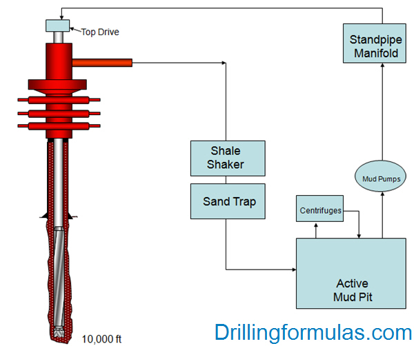
Lag time is traveling time interval required for pumping cuttings from each particular depth to surface. It can be expressed in terms of time (minutes) and pump strokes.


The lag time always changes when a well becomes deeper and/or pumping speed change. Two factors, affecting lag time calculation, are annulus volume of drilling fluid in and drilling mud flow rate.

With certain annular volume, the lag time, normally expressed in minutes, can be determined by dividing the annular volume (bbls) by the flow rate (bbl/min).

If there are changes in mud flow rate, the lag time figure will be changed as well. In order compensate for any changes, the lag time is transformed into pump strokes too; therefore, a change in speed of pump will not affect the lag time.

How to Calculate Theoretical Lag Time

There are 3 steps to do in order to calculate lag time as listed below;

1. Calculate pump output
2. Calculate annula
r volume at certain depth of hole
3. Calculate the theoretical lag time

Oilfield Unit

Example – Determine lag time from bottom to surface with the following information;

Bit depth = 9500’ MD
Pump rate = 300 GPM
Annular volume at 9500’ MD = 250 bbl
Triplex pump output = 0.102 bbl/stroke

Solution;

Pump rate = 300 GPM ÷ 42 = 7.14 bbl / minute
Lag time in minutes = 250 bbl ÷ 7.14 bbl / minute = 35 minutes
Lag time in strokes = 250 bbl ÷ 0.102 bbl/stroke = 2451 strokes

Metric Unit

Bit depth = 3,300 m
Pump rate = 1,200 liter/min
Annular volume at 3,300 m = 40 m3
Triplex pump output = 0.01622 m3/stroke

Solution;

Lag time in minutes = 40 m3 ÷ (1,200 ÷ 1,000 m3/ min) = 33.3 minutes
Lag time in strokes = 40 m3 ÷ 0.01622 m3/stroke = 2466 strokes

Download Lag Time Calculation Spreadsheet

Ref books: 

Lapeyrouse, N.J., 2002. Formulas and calculations for drilling, production and workover, Boston: Gulf Professional publishing.

Bourgoyne, A.J.T., Chenevert , M.E. & Millheim, K.K., 1986. SPE Textbook Series, Volume 2: Applied Drilling Engineering, Society of Petroleum Engineers.

Mitchell, R.F., Miska, S. & Aadny, B.S., 2011. Fundamentals of drilling engineering, Richardson, TX: Society of Petroleum Engineers.

Boyle’s Gas Law and Its Application in Drilling

Understand Boyle’s Gas Law

Boyle’s gas law states that at constant temperature, the absolute pressure and the volume of a gas are inversely proportional in case of constant temperature within a closed system.  Bolye’s law can be illustrate in the graph shown in figure 1.

Figure 1 – Boyle’s Law

Well, we can describe the statement above into simple mathematics as following formula:

Boyle’s Gas Law

P x V = constant

Or express Boyle’s law in another term:

P1 x V1 = P2 x V2

Where;

P1 = Pressure at condition # 1

 V1 = Volume at condition # 1

P2 = Pressure at condition # 2

 V2 = Volume at condition # 2

Note: You can use any unit for Bolye’s gas law as long as P1 and P2 are the same unit and V1 and V2 are the same unit.

Let’s apply Boyle’s law into our drilling business

Calculate the volume of gas you will have on the surface, 14.7 psi for atmospheric pressure, when 1 bbl of gas kick is circulated out from reservoir where has formation pressure of 3,000 psi. Figure 2 and 3 shows the condition of this well.

Figure 2 – Gas Kick 1st condition at the bottom

Figure 3 – Gas Kick 2nd condition

Apply the Boyle’s Gas Law:

P1 x V1 = P2 x V2

P1= 3000 psi (reservoir pressure)

V1 = 1 bbl (volume at bottom hole)

P2 = 14.7 psi (atmosphere pressure)

V2 = ? (volume at surface)

P1 x V1 = P2 x V2

3000 x 1 = 14.7 x V2

V2 = 204 bbl

Figure 4 – Gas

References

Cormack, D. (2007). An introduction to well control calculations for drilling operations. 1st ed. Texas: Springer.

Crumpton, H. (2010). Well Control for Completions and Interventions. 1st ed. Texas: Gulf Publishing.

Grace, R. (2003). Blowout and well control handbook [recurso electrónico]. 1st ed. Paises Bajos: Gulf Professional Pub.

Grace, R. and Cudd, B. (1994). Advanced blowout & well control. 1st ed. Houston: Gulf Publishing Company.

Watson, D., Brittenham, T. and Moore, P. (2003). Advanced well control. 1st ed. Richardson, Tex.: Society of Petroleum Engineers.