


When you learn about drilling mud, the rheological models are essential knowledge. The rheological models are critical for a drilling fluid study because they are used to simulate the characteristics of drilling mud under dynamic conditions. With this knowledge, you will be able to determine some of the key figures, such as equivalent circulating density, pressure drops in the system, and hole cleaning efficiency.
The drilling fluid has three flow regimes, plug flow, laminar flow and turbulent flow and Figure 1 demonstrates 3 flow regimes on the shear rate and shear stress curve. In between each zone, there is a transition zone where the flow regimes are changing.

Figure 1 – Various flow types
Plug Flow
Plug flow happens only with a very low shear rate and when the mud is in a gel stage. The velocity of the mud at the center of the annulus is equal to the velocity at the sides.
Laminar Flow
The laminar flow usually occurs at a low flow velocity and it is best understood by considering mud as being layers of fluid flow. The velocity of the mud in the center is moving the fastest and the velocity of an adjacent layer moves slower. At the edge of the pipe, the velocity is very low when compared to the velocity in the center. For the laminar flow, the flow has a predictable pattern, and the shear rate is a function of the shear stress of the fluid. Therefore, the equations used for the laminar flow are based on fluid flow models, such as Newtonian, Bingham Plastic, and Power Law.
Turbulence Flow
Fluid moving in a turbulence flow region is subject to random local fluctuations in both the direction of flow and fluid velocity. For the turbulent flow, it is difficult to find the proper equations to describe the fluid flow models because the flow at this stage is disorderly. Practically, most people use empirical equations to figure out the flow relationship for this flow regime.
Things to remember include that the drilling mud does not follow each particular fluid model exactly; however, either one or more fluid models can be utilized to predict the flow behavior of drilling mud and as a result it is still within a reasonable range.
Rheology models that you need to understand are Newtonian, Bingham Plastic, Power Law and Hershel-Bulkley.
Newtonian Fluid Model
A Newtonian fluid model is the simplest model. Let’s describe it in a mathematical way, a relationship between shear stress (lb/100 ft2) and shear rate (1/sec), which is called a consistency curve, is a straight line which passes through the original (see the figure below).
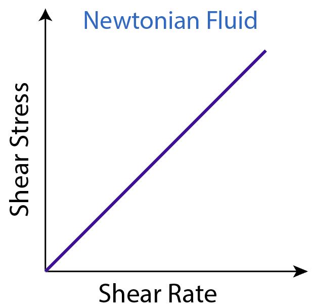
Figure 2 – Newtonian Fluid Model
What’s more, viscosity of the Newtonian fluid is the slope of the consistency curve. The Newtonian fluid has a single viscosity value for every shear rate.
Which fluid is classified as the Newtonian fluid?
The fluid that has particles no larger than the fluid molecule can be applied to the Newtonian model to predict flow behavior. For example, light oil, water, and salt solution are all examples of a Newtonian fluid.
Newtonian fluid does not represent the behavior of drilling fluid because viscosity does not change by shear rate. However, drilling fluid is far more complex than a simple Newtonian fluid behavior and individual drilling fluids vary considerably in their flow behavior. The biggest difference between Newtonian fluid and drilling mud is the reactions between fine particle suspensions in the mud.
Figure 3 demonstrates differences between Newtonian fluid and drilling mud in a shear rate and shear stress plot. Two major points illustrated from the Figure 3 are as follows;
- Curve of drilling mud is not in a straight line. It means that viscosity is not a constant value.
- Shear stress is not zero at a zero shear rate.
In drilling fluid, there is some internal resistance to overcome in order to move fluid from a static condition. The graph (Figure 3) clearly shows that there is no fixed value for mud viscosity, but it tends to become lower as shear rate increases.
Note: viscosity = shear stress ÷ shear rate
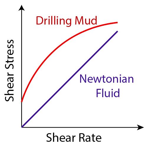
Figure 3 – Drilling Fluid Vs Newtonian Fluid
Bingham Plastic Model
The most commonly used fluid model to determine the rheology of non-Newtonian fluid is the Bingham plastic model. With this model, it makes the assumption that the shear rate is a straight line function of the shear stress. The point where the shear rate is zero is called “Yield Point” or threshold stress. Furthermore, the slope of the shear stress and the shear rate curve is called “Plastic Viscosity.” Bingham plastic model produces acceptable results for a drilling mud diagnosis, whereas, it is not accurate enough for hydraulic calculations.
Plastic Viscosity (PV) can be determined by the following formula;
Plastic Viscosity (PV) = reading at 600 rpm – reading at 300 rpm
Yield Point (YP) can be determined by the following formula;
Yield Point (YP) = reading at 300 rpm – Plastic Viscosity (PV)
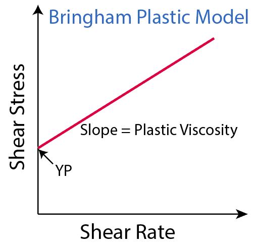
Figure 4 – Bingham Plastic Model
Power Law Model
The power law model is another fluid model used to describe a characteristic of non-Newtonian fluid in which the shear stress and shear rate curve, called “a consistency curve,” has the exponential equation as described below:
Shear Stress = K x (shear rate)n
Where;
K is the fluid consistency unit.
n is the power law exponent.
Using a viscometer to measure shear stress at 600 and 300 rpm and use these figures to calculate n and K by these following equations.
n = 3.32 log (reading at 600 ÷ reading at 300)
K = 5.11 (reading at 300 ÷ 511n)
According to the equations, the relationship between the shear stress and the shear rate can be constructed like it is in Figure 5.
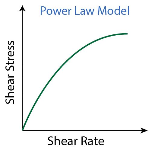
Figure 5 – Power Law Model
The drawback of the Power Law fluid model is that at zero shear rate, the shear stress is zero. This does not truly represent drilling mud because drilling mud has a residual shear strength at a zero shear rate.
Herschel Bulkley
The Herschel Bulkley is an improvement model from Power Law fluid model in order to match the actual behavior of drilling fluid at a low shear rate by assuming an initial shear stress value. Herschel Bulkley can be described as per the equation below;
Shear Stress = Yield Stress + K x (shear rate)n
Where;
K is the fluid consistency unit.
n is the power law exponent.
The yield stress is normally taken from value of 3 rpm reading and the n and K values are calculated from the 600 or 300 rpm values or they can be interpolated using mathematical method from a graph. Figure 6 represents the Herschel Bulkley Model.

Figure 6 – Herschel Bulkley Model
Note: Newtonian fluid n = 1 and there is no shear stress at a zero shear rate. For drilling mud, n is always less than 1 and there is shear stress at a zero shear rate which is called “Yield Stress.”
References

